EUCLIPSE

Introduction and motivation

Marine stratocumulus (Scu) clouds strongly influence the radiative budget of the Earth. Predicting how both their geographical distribution and their physical properties would respond to climate change is still a fundamental open question. At the same time the subtle and complex interaction between atmospheric dynamics and convective, turbulent and radiative processes, from which Scu arise, is difficult to be captured by a general circulation model (GCM). For these reasons the Scu, together with cumulus clouds, are still the heart of the problem of climate feedback uncertainties, as claimed in Bony and Dufresne (2005).

Recently many efforts are put into identifying the causes of the large model spread for low-cloud climate feedback. In particular CGILS project is a Single-Column Model (SCM) and Large Eddy Simulation intercomparison study aimed to investigate this issue. The set-up includes three cases corresponding to three cloud regimes: coastal stratus (S12), Scu (S11) and cumulus (S6). The idealized large-scale forcings and free-tropospheric conditions are based on selected locations along the GPCI transect. The models are forced to a steady-state for the control set-up and the for perturbed large-scale conditions, mimicking climate change. The response to this perturbation gives information on the feedback. On the one hand LESs agree well in the sign of the feedback, while SCM spread is still significant [Zhang and Bretherton 2008, Zhang and co-authors 2012, Blossey et al. 2012].

The present framework is aimed to be a CGILS extension. In particular we generalize the Scu steady-state response to climate change for different meteorological conditions. The scientific questions we want to address are the following:

1. What are the steady-state solutions of a Scu-topped atmospheric boundary layer (ABL) for a wide range of different atmospheric conditions?
2. How are the steady-state solutions affected by perturbations of large-scale (LS) forcing?

Set-up philosophy

As in CGILS the model is forced with idealized conditions that represent the summer climatology of the North-East Pacific. In order to make the set-up flexible and robust we need to simplify the atmospheric characteristic. In particular we neglect the horizontal advection and the diurnal cycle by keeping constant the solar incoming short-wave radiation. According to this assumptions the free-tropospheric conditions are defined in order to reach an equilibrium. We are interested in assessing the response of atmospheric boundary layer to free-tropospheric conditions. To this end we consider different profiles which are at the same time realistic for the Scu region and coherent with our assumptions. In this way the thermodynamic jumps at the inversion top vary systematically. An ad-hoc defined phase space is used for analysing the results.

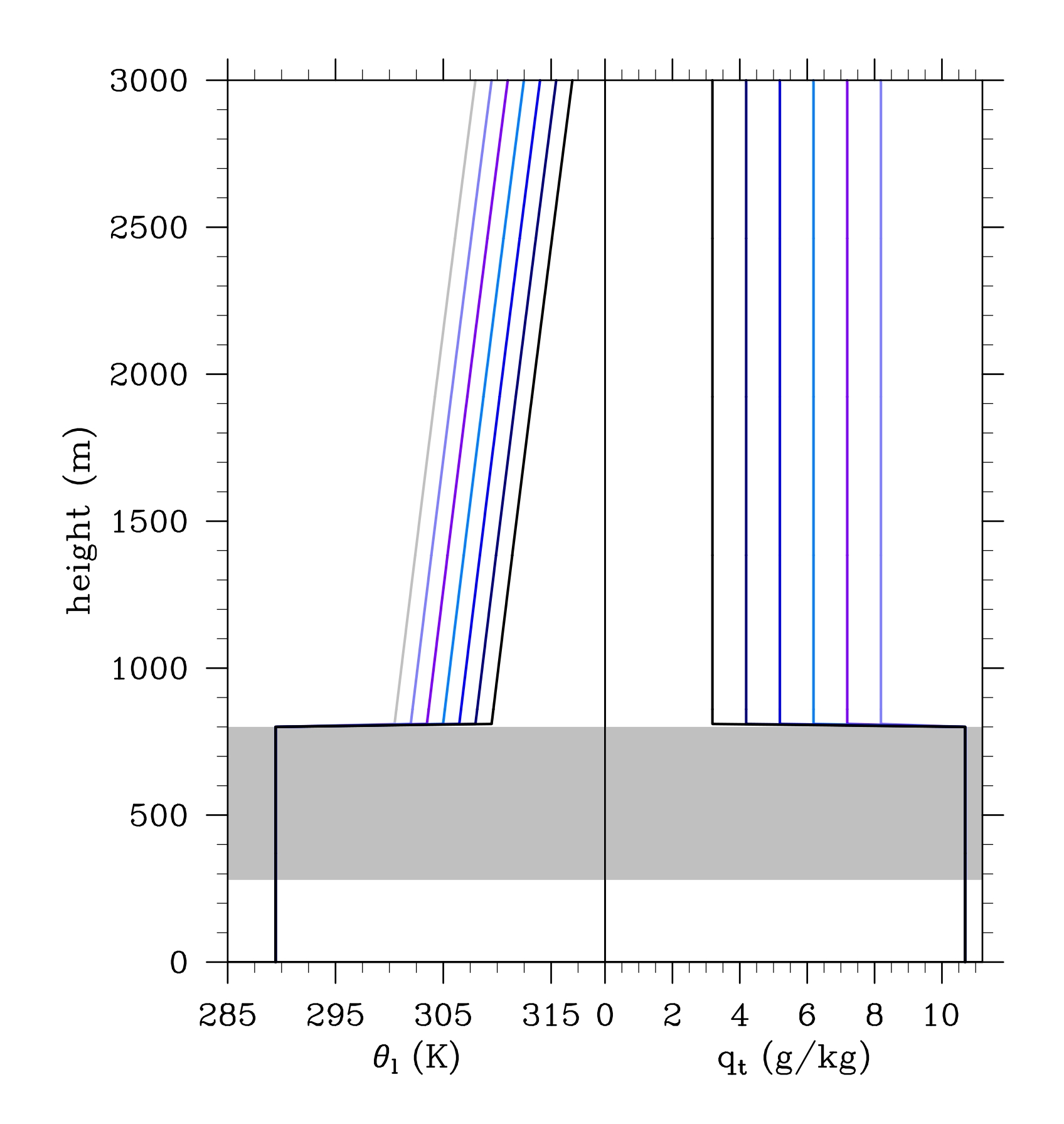
Figure 1: initial conditions of CTL case: some examples of liquid water potential temperature, θl, and total water content,qt , profiles. The grey zone represents the cloud layer.

Subsequently we perturb the large-scale forcing in order to mimic the climate change. The considered perturbation consists of a sea surface temperature increase of 2 K. The free tropospheric thermodynamic profiles are defined according to the hypotheses of globally uniform warming of the oceans and unperturbed relative humidity distribution. The ABL response gives information on the cloud-climate feedback.

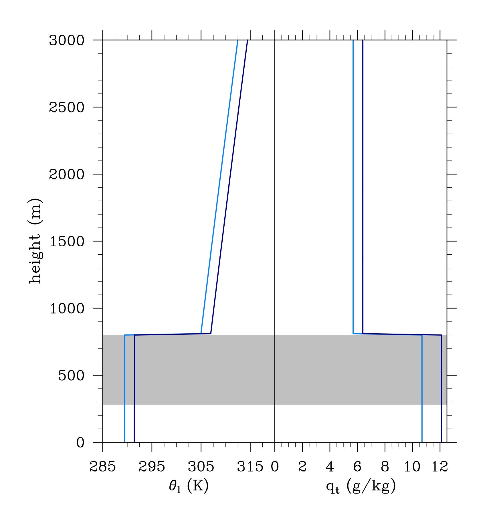
Figure 2: comparison between initial thermodynamic profiles of CTL (light blue) and perturbed climate (PC) case (dark blue): examples of liquid water potential temperature, θl, and total water content, qt. The grey zone represents the cloud layer.

The proposed framework has been already used for both Mixed-Layer Model and Single Column Model studies [de Roode et al (2012), Dal Gesso et al (2013a), Dal Gesso et al (2013b)]. We believe that it is a powerful tool for both gaining insight in the physical processes that determine the cloud-climate feedback and testing the skills of different models in representing cloud-climate interaction. For this reason the present intercomparison study has been set-up within wp3 of EUCLIPSE project.

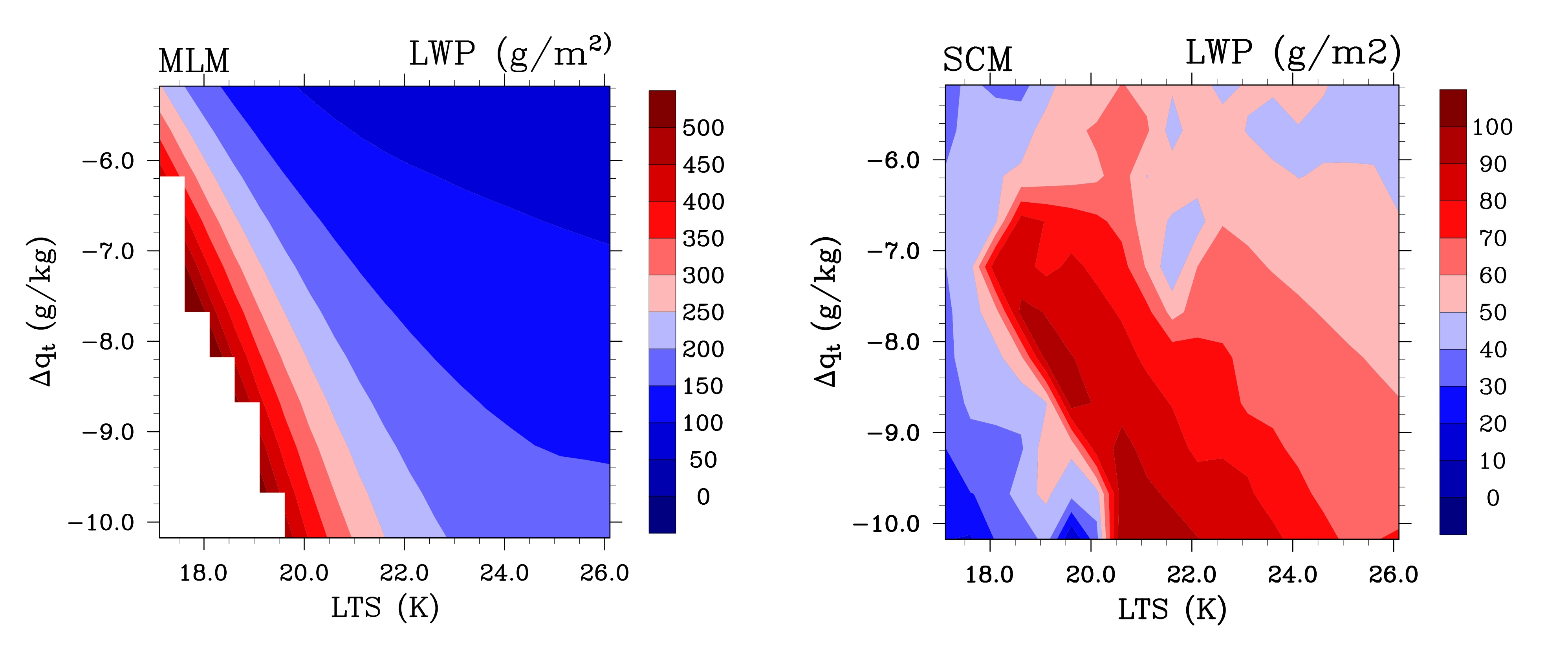
Figure 3: results of previous studies which applied the present framework: liquid water path (LWP) pattern in the phase space defined by lower tropospheric stability (LTS) and a similar bulk jump for humidity. The left panel shows results obtained with a non-precipitating Mixed-Layer Model (MLM) coupled with Nicholls and Turtons entrainment parametrization and the right panel shows the rusults obtained with Single-Column Model (SCM) version of RACMO.

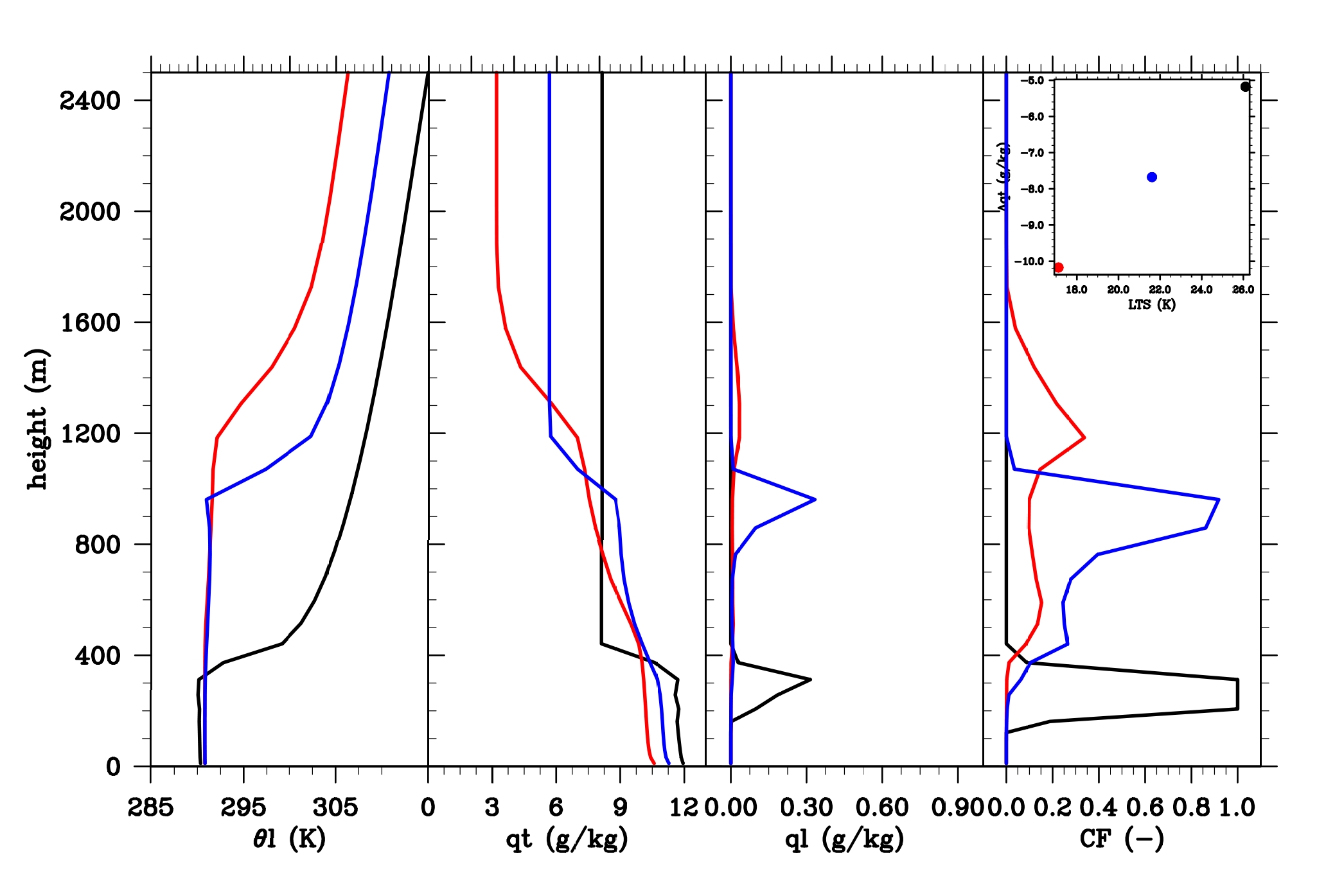
Figure 4: θl, qt, ql and CF vertical profiles of three selected cases along the diagonal of the maximum variation on LWP. The characteristic profiles of the Scu to cumulus transition are found.

Schedule

For information and suggestions please email Sara Dal Gesso, Pier Siebesma and Stephan de Roode. Simulation results should be upload via FTP, to receive your personal account send an email to the following email address: filexchange@vrlab.tudelft.nl. The intercomparison study deadline is October 15, 2013.

Documentation

A complete desciption of this intercomparison study can be downloaded here.

A folder contaning explicit initial profiles is stored here. The folder contains four NetCDF files: two with the initial conditions for the CTL (SteadyStates_CTL_input.nc) and the PC case (SteadyStates_PC_inprof.nc) and two containing the transient forcing for the CTL (SteadyStates_CTL_SF_input.nc) and PC (SteadyStates_PC_SF_inprof.nc) case.

Results

The results of the first phase of the intercomparison study have been reported in an article under revision in JAMES. The results of SCM and LES simulations are available in the section Results of this webpage.