EUCLIPSE

 

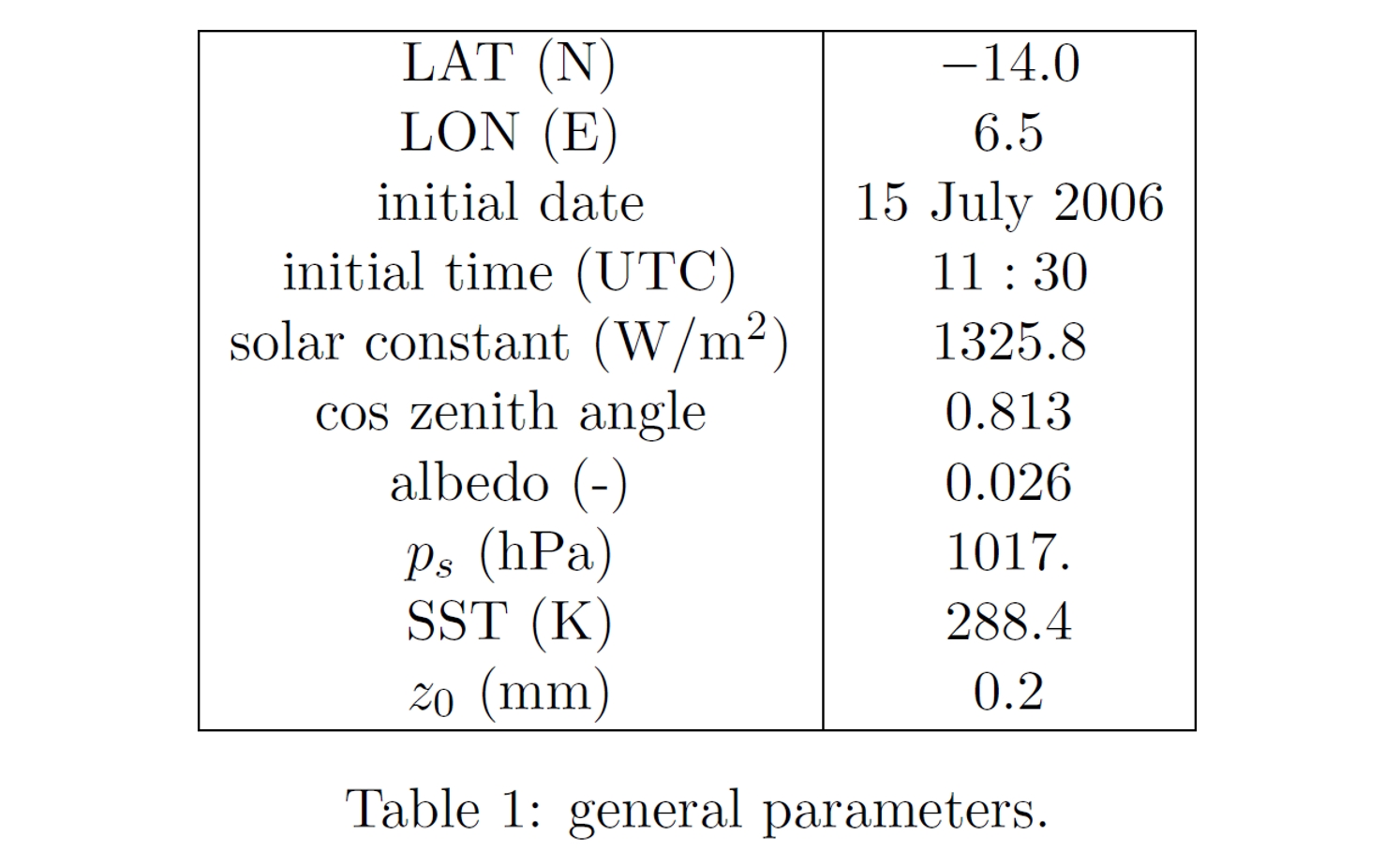
The simulations start at local noon on 15 July 2006 and last just one time-step. They are located at coordinate 14.0 S and 6.5 E. For further details, see Table 1.

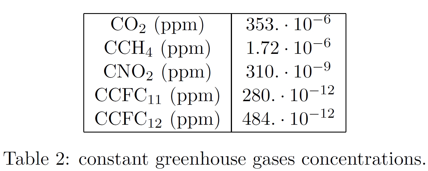
If possible we ask for using the constant greenhouse gases concentrations provided in Table 2 (since the ozone concentration is height dependent, it is contained in the NetCDF file).

All the necessary informations are collected in the NetCDF file radiationtest_input.nc.

Initial conditions

The initial profiles are based on standard atmosphere characteristics and on observations.

Boundary Layer: 0. < z < 600. m
In order to obtain different amounts of liquid water path (LWP), the liquid water equivalent potential temperature, θ_l, has been maintained constant while for the total water content, q_t, a value belonging to the following set has been chosen:
θ_l = 287.5 K
q_t = (8.00; 8.50; 8.57; 8.64;8.71; 8.78; 8.85; 8.92; 8.99; 9.06; 9.40; 9.17; 9.30; 9.43; 9.56; 9.69; 9.82; 9.95) g/kg
The first profile corresponds to the clear sky case while the others correspond to a stratocumulus clouds topped boundary layers with increasing LWP.

Figure 3: profiles of potential temperature (on the left) and temperature (on the right) in the boundary layer.

Figure 4: profiles of total water content (on the left) and liquid water content (on the right) in the boundary layer

Free Tropophere: 600. < z < 16250. m
T = (-6.55946 K/km) z + (302.455 K)
RH = 0.15

Tropopause: 16250. < z < 24700. m
T = (3.40457 K/km) z + (138.474 K)
q_t = 0. g/kg

Stratosphere:
q_t = 0. g/kg

• 24700. < z < 30650. m: T = 222.5 K
• z > 30650. m: T = (- 1. K/km) z + (253.32 K)

Figure 5: profiles of potential temperature (on the left) and total water content (on the right) up to the top of the atmosphere.

Microphysics

 In order to study the various impacts of the cloud microphysical assumptions we ask for three different sets of simulations.<\p>

 As a first experiment (SET A) we ask for results obtained by simply using the default operational setup of the model as they are used in the CMIP5 climate model runs. This is useful to assess how the various radiation codes will respond to stratocumulus fields in their operational setting, in which they often assume a simple climatology for their effective radius and sometimes assume a fixed inhomogeneity factor to take spatial inhomogeneity of the LWP into account.<\p>

 In the second experiment (SET B) we ask to constrain the cloud microphysics through assuming no spatial inhomogeneity in the liquid water content. So models that are employing an inhomgeneity factor are asked to set this to 1. Furthermore we assume no dispersion in the cloud droplet distribution (i.e. all the droplets have the same prescribed radius at a given height). A further common (but not so realistic) hypothesis in climate and NWP models is that the effective radius is constant with height in stratocumulus. We therefore require a constant effective radius with height which is set equal to 9. μm, according to SEVIRI observations. 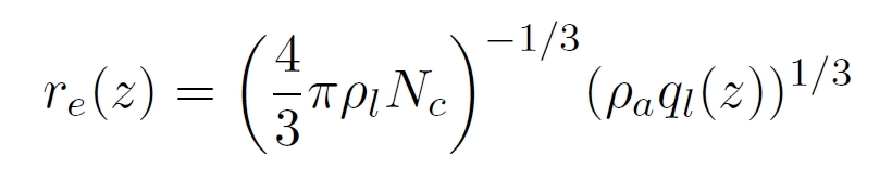This implies that the cloud droplet number concentration, N_c, varies with height as follows:

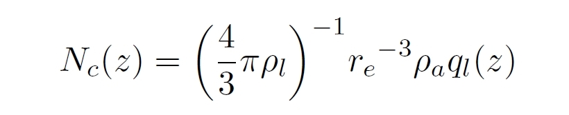
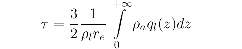
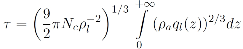
where ρ_a is the air density, ρ_l the liquid water density and q_l the liquid water content.
With these assumptions the optical depth, τ , reads as

 Finally, as a more realistic variation on the second experiment, we require in the third experiment (SET C) a constant cloud droplet number concentration: N_c = 200. cm-3. Along with the previous assumptions of non-dispersive delta-peaked distribution of the cloud droplet size distribution and no inhomogeneity for the liquid water content, this leads to an effective radius which is height dependent

and an optical depth given by

 The description of the intercomparison study sets can thus be summarized as:

• SET A: operational set-up;
• SET B: prescribed effective radius: r_e = 9 μm;
• SET C: constant cloud droplet number concentration: N_c = 200. cm-3.

Vertical resolution

 Since vertical resolution might influence the results substantially we require that radiation codes run as Single Column Model versions of climate and numerical weather prediction models provide results at two different resolutions:

• the standard resolution such as used in the operational runs;
• a higher prescribed resolution.

The higher prescribed resolution is defined by the hybrid coordinate constants A's and B's, that determine the pressure at the model half levels through:
p_k+1/2 = A_k+1/2 + B_k+1/2 p_s
where p_s is the prescribed surface pressure. The A's and B's are provided in the NetCDF file radiationtest_input.nc.

Radiation codes that run in LES models should run at a vertical resolution of 10 m in the lowest 1 kilometer. Beyond this height the resolution can be made coarser through the use of a stretched grid.